From Theory to Reality: Understanding Machine Learning with ML.NET

Machine learning uses algorithms to learn.

Great, but how? How does it use these algorithms and which algorithm does what?

Let’s break down some of the core concepts that power these intelligent algorithms, starting with one of the most important: Gradient Descent.

Gradient Descent: The Climb Down

Think of gradient descent like hiking down a mountain in the fog. You can't see the whole path, but with every step, you feel for the steepest way down. Our goal is to reach the base of the mountain.

Using Gradient Descent, the algorithm tweaks the model parameters with each step to minimize the errors between predictions and actual outcomes. In other words, the model learns by trial and error, adjusting weights to minimize the mistakes it makes during training.

Regularization: Controlling Model Complexity

Imagine you’re building a house of cards. If you make it too complex, it’s likely to collapse. In machine learning, regularization prevents models from becoming too complicated (overfitting the training data) by penalizing large coefficients. This keeps the model general enough to work well with unseen data.

Regularization helps maintain a balance between simplicity and accuracy, preventing models from becoming overly complex.

Neural Networks: Mimicking the Brain

Neural networks are like interconnected webs of neurons in the human brain. Each node (or "neuron") processes input and passes it forward, learning complex patterns from the data. These networks shine when the relationships between data points are non-linear and intricate, such as in image or speech recognition tasks.

Neural networks are powerful tools for recognizing patterns and handling complex data relationships, much like the way our brains process information.

Decision Trees: Breaking Down Decisions

A decision tree is like a flowchart where each internal node represents a decision based on a feature, and each leaf represents an outcome. It’s a simple yet effective way of breaking down decisions. Decision trees are particularly useful when interpretability is important. They make it easy to break down decisions step by step, offering a simple and intuitive way of making predictions.

Bringing It All Together

House Price Prediction Model with ML.NET

Let’s build a machine learning model to predict house prices based on various features such as the size of the house, number of bedrooms, and location. This will allow us to bring together all the concepts we discussed earlier and see them in action using ML.NET.

We’ll create a simple console app and apply these methods to our dataset to see how they are different. We are going to use ML.NET as much as we can, and when we cannot, we’ll call the Python code to do the work for us.

Setting Up the Data

We’ll start with a simple dataset containing historical house prices and features like the number of bedrooms, size in square feet, and location (in the form of zip code). Here’s how to load the data into ML.NET:

var mlContext = new MLContext();
var dataView =
 mlContext.Data.LoadFromTextFile<HouseData>("VirtualTownHouseDataset.csv", 
    hasHeader: true, separatorChar: ',');

Our dataset, VirtualTownHouseDataset.csv, is a made-up dataset. I used ChatGPT to make this data for me and it has 5,000 rows in it.

HouseData that you see in the code above is a class that represents each row in the dataset:

csharpCopy codepublic class HouseData
{
    public float Size { get; set; }
    public float Bedrooms { get; set; }
    public float Price { get; set; }
    public string ZipCode { get; set; }
}

Step 2: Preprocessing and Feature Engineering

We need to transform the categorical data (ZipCode) into numeric form and normalize the features so the model can process them properly:

 var preprocessingPipeline = mlContext.Transforms.Categorical.OneHotEncoding("ZipCode")
   .Append(mlContext.Transforms.Concatenate("Features", "Size", "Bedrooms", "ZipCode"))
   .Append(mlContext.Transforms.NormalizeMinMax("Features"));

The code above creates a preprocessing pipeline in ML.NET to prepare our raw data before feeding it into a machine learning model.

You may notice a somewhat foreign keyword called OneHotEncoding. This is a technique used to convert categorical (non-numeric) variables into a format that can be provided to machine learning algorithms to improve their performance. In our case, ZipCode is converted into multiple binary columns each representing a unique ZipCode.

For example, when we have values like, "12345", "67890", "11223", after one-hot encoding, the resulting features will look like:

[1, 0, 0] for "12345"
[0, 1, 0] for "67890"
[0, 0, 1] for "11223"

Then we concatenate all individual features (such as Size, Bedrooms etc.) and our one-hot encoded ZipCode column into a single column called Features. This column is going to be used to train our model.

Then we apply Min-Max normalization to scale all features to a common range. After this transformation, all columns in the Features vector will have values between 0 and 1.

It is now time to train our model with different algorithms.

Step 3: Training with Gradient Descent and Regularization

To train a model using gradient descent and apply regularization to avoid overfitting, we can use the SDCA regression trainer in ML.NET. This will give us a linear regression model:

 public static void RunSdcaRegression(MLContext mlContext, IEstimator<ITransformer> preprocessingPipeline,
        IDataView dataView)
    {
        var pipeline = preprocessingPipeline.Append(mlContext.Regression.Trainers.Sdca(
            "Price", l2Regularization: 0.1f)); // L2 Regularization to prevent overfitting

        var model = pipeline.Fit(dataView);
        var predictions = model.Transform(dataView);
        var metrics = mlContext.Regression.Evaluate(predictions, "Price");
        Console.WriteLine("=== Gradient Descent (SDCA) Results ===");
        Console.WriteLine(
            $"R^2: {metrics.RSquared}, MAE: {metrics.MeanAbsoluteError.ToString("N2", CultureInfo.InvariantCulture)}");
        MakePrediction(mlContext, model);
    }

The L2 regularization prevents the model from overfitting by penalizing large coefficient values. This keeps the model simpler and more generalizable.

Step 4: Adding a Decision Tree

For comparison, we can also train a decision tree model using the FastTree algorithm. Decision trees often perform well on structured data with clear feature splits:

public static void RunFastTreeRegression(MLContext mlContext, IEstimator<ITransformer> preprocessingPipeline,
        IDataView dataView)
    {
        var pipeline = preprocessingPipeline.Append(mlContext.Regression.Trainers.FastTree("Price"));

        var model = pipeline.Fit(dataView);
        var predictions = model.Transform(dataView);
        var metrics = mlContext.Regression.Evaluate(predictions, "Price");
        Console.WriteLine("=== Decision Tree (FastTree) Results ===");
        Console.WriteLine(
            $"R^2: {metrics.RSquared}, MAE: {metrics.MeanAbsoluteError.ToString("N2", CultureInfo.InvariantCulture)}");
        MakePrediction(mlContext, model);
    }

This gives us a different perspective: instead of optimizing through gradient descent, the decision tree splits the dataset into smaller subsets based on feature thresholds.

Step 5: Experimenting with Neural Networks

For more complex relationships, we can also experiment with a neural network.

However, we hit a glitch here. ML.NET is great for many traditional machine learning tasks like linear regression, decision trees and clustering but it lacks built-in tools to create and train complex neural networks.

Neural networks, especially deep learning models with multiple layers, require a framework that supports building and training those layers, and ML.NET is not designed to handle that.

Azure Machine Learning is also not a good fit because it is mostly used for training models at a large scale using cloud resources. On top of that, running neural networks in Azure is often more expensive and more complicated to setup and run involving many steps compared to running a local Python script. It is an overkill in our case.

For the reasons above, we run a local Python script since Python has frameworks like TensorFlow and Keras that are specifically made for creating and training neural networks. Once you look at the code in Python script, you’ll appreciate why Python is the go-to language for deep learning.

To run a Python script from a C# project, we add a class to our project called NeuralNetworkPredictorPythonScript and then we call it from our main program.

This class is responsible for running the script using a Python interpreter (in this case, the python.exe from my virtual environment), then getting the result from the script in JSON format and displaying it in our app.

public PredictionResult? PredictHousePrice(double size, int bedrooms, string zipCode)
    {
        var processStartInfo = CreateProcessStartInfo(size, bedrooms, zipCode);

        try
        {
            using var process = Process.Start(processStartInfo);
            if (process == null)
            {
                LogError("Failed to start Python process.");
                return null;
            }

            var (output, errors) = GetProcessOutput(process);
            LogErrors(errors);

            if (string.IsNullOrEmpty(output))
            {
                LogError("No output received from Python script");
                return null;
            }

            return ParsePredictionOutput(output);
        }
        catch (Exception ex)
        {
            LogError($"Error running Python script: {ex.Message}");
            return null;
        }
    }

Our process start info:

private ProcessStartInfo CreateProcessStartInfo(double size, int bedrooms, string zipCode)
    {
        return new ProcessStartInfo
        {
            FileName = _pythonPath,
            Arguments = $"\"{_scriptPath}\" {size} {bedrooms} {zipCode}",
            RedirectStandardOutput = true,
            RedirectStandardError = true,
            UseShellExecute = false,
            CreateNoWindow = true,
            WorkingDirectory = _workingDirectory,
            StandardOutputEncoding = Encoding.ASCII,
            StandardErrorEncoding = Encoding.ASCII,
            EnvironmentVariables =
            {
                ["TF_CPP_MIN_LOG_LEVEL"] = "3",
                ["TF_ENABLE_ONEDNN_OPTS"] = "0",
                ["PYTHONIOENCODING"] = "ascii"
            }
        };
    }

pythonPath is where your python.exe is and scriptPath is where your script is located at - in this case it is at the root directory of our project, so we define it as:

public NeuralNetworkPredictorPythonScript(string pythonPath = "")
    {
        _pythonPath = !string.IsNullOrEmpty(pythonPath)
            ? pythonPath
            : Environment.GetEnvironmentVariable("EnvPython312") 
                ?? @"C:/YourDefaultPythonPath/python.exe";
        _workingDirectory = Directory.GetCurrentDirectory();
        _scriptPath = Path.Combine(_workingDirectory, "HousePriceNeuralNetwork.py");
    }

One gotcha here is to make sure that you have all the frameworks and libraries installed in your virtual environment.

💡

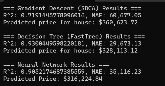
If you want a refresher on how to create a virtual environment in Windows for Python, please see my article:

When we run our program, we get the predicted house pricing for all 3 methods:

Why are the results different and what are R², MAE

When you look at the results above, there are 3 questions we can ask:

What is R²?
What is MAE?
Why are the prices so different?
How do I know which one to use?

OK, 4 questions.

Let’s go through them and see what is going on.

What is R²?

R², is a scale from 0 to 1 or 0% to 100%. It means how much of the price variations the model can explain. For example, an R² of 0.93 means the model can explain 93% of why house prices are different from each other. Naturally, higher is better.
What is MAE?

MAE stands for Mean Absolute Error, and its scale is the same as the price (dollars in this case), indicating how far off the predictions are. For example, a MAE of 32,500 means predictions are off by about $32,500 on average. In this case, lower is better.
Why are the prices so different?

Each algorithm uses a different approach to learn from data.

SDCA uses linear relationships which is good at finding linear patterns and it trades accuracy for simplicity.

FastTree is good at creating decision boundaries, and handling categorical data and it trades interpretability (understandability) for accuracy.

Neural Networks are good at finding complex patterns and try to balance both, but they require more computational resources. When you run the program, you will realize that while the first two algorithms run pretty fast, the last one takes its time (it runs through 100 iterations to learn - that’s what the epochs=100 is for in the Python code).
How do I know which one to use?

The answer to that question really depends on what you need. If you need interpretability, then SDCA might be better. If you have complex relationships and need scalability, then a Neural Network is your answer. If you need raw accuracy, then FastTree is your best friend.

In our case above, FastTree appears to be the best model to use because it has the highest R² value (0.93) and lowest MAE ($29,673), which means it makes the smallest average errors. These numbers suggest it’s capturing the relationships in the data most accurately.

Conclusion

If you need a single model, it appears that using the FastTree model gives you the best performance metrics.

In the real world, you would combine multiple models, collect more training data, use cross-validation to ensure consistent performance, and monitor model performance over time.

On top of that, you would compare your results with actual market prices in the area, get domain expert validation, and consider using confidence intervals or prediction ranges. *

By comparing these different machine learning algorithms in the context of a single problem—predicting house prices—we can see how gradient descent, decision trees, and neural networks work and how they all have unique strengths. The key is finding the right balance of complexity and accuracy for your particular dataset.

Here is the link to the GitHub project:

* Confidence intervals and prediction ranges mean that instead of predicting a single price, we could express it as a range. For example, if we were to use our best model’s results from above, our predicted price is $328,113 with a MAE of $29,673. Therefore, we say "We predict this house will sell for between $298,440 and $357,786". In our example, we are 68% confident about this price.

Why the number 68?

The number 68 comes from statistics. If you plot prediction errors in most machine learning models, they tend to follow a bell curve pattern where:

About 68% of values fall within ±1 standard deviation (or in our case, ±1 MAE)
About 95% fall within ±2 standard deviations (±2 MAE)
About 99.7% fall within ±3 standard deviations (±3 MAE)

This is known as the "68-95-99.7 rule" or the "empirical rule" in statistics.

If we were to apply this to our data, we get:

95% confidence: $328,113 ± (2 × $29,673) = $268,767 to $387,459
99.7% confidence: $328,113 ± (3 × $29,673) = $239,094 to $417,132

The tradeoff is that the higher the confidence, the wider the range, which is less precise but more likely to be correct.

From Theory to Reality: Understanding Machine Learning with ML.NET

Comments

Machine Learning Fundamentals

Evaluating and Tuning the Model in Machine Learning

More from this blog

Assembly vs Modern Languages

MCP Server: Standardizing LLM API Calls

Building Your First Model Context Protocol Server in C#

Kubernetes Without The Tears — A 7-Day Developer Journey

Day 7 - Kubernetes Without The Tears

Gradient Descent: The Climb Down

Regularization: Controlling Model Complexity

Neural Networks: Mimicking the Brain

Decision Trees: Breaking Down Decisions

Bringing It All Together

Setting Up the Data

Step 2: Preprocessing and Feature Engineering

Step 3: Training with Gradient Descent and Regularization

Step 4: Adding a Decision Tree

Step 5: Experimenting with Neural Networks

Why are the results different and what are R², MAE

Conclusion

Command Palette

Comments

Machine Learning Fundamentals

Evaluating and Tuning the Model in Machine Learning

More from this blog

Gradient Descent: The Climb Down

Regularization: Controlling Model Complexity

Neural Networks: Mimicking the Brain

Decision Trees: Breaking Down Decisions

Bringing It All Together

Setting Up the Data

Step 2: Preprocessing and Feature Engineering

Step 3: Training with Gradient Descent and Regularization

Step 4: Adding a Decision Tree

Step 5: Experimenting with Neural Networks

Why are the results different and what are R², MAE

Conclusion